Acoustic Scattering - Maze

One line description of the data: Simple acoustic wave propogation through maze-like structures.

Longer description of the data: These variable-coefficient acoustic equations describe the propogation of an acoustic pressure wave through maze-like domains. Pressure waves emerge from point sources and propogate through domains consisting of low density maze paths and orders of magnitude higher density maze walls. This is built primarily as a challenge for machine learning methods, though has similar properties to optimal placement problems like WiFi in a building.

Domain expert: Michael McCabe, Polymathic AI.

Code or software used to generate the data: Clawpack, adapted from this example.

Equation:

\[ \begin{align*} \frac{ \partial p}{\partial t} + K(x, y) \left( \frac{\partial u}{\partial x} + \frac{\partial v}{\partial y} \right) &= 0 \\ \frac{ \partial u }{\partial t} + \frac{1}{\rho(x, y)} \frac{\partial p}{\partial x} &= 0 \\ \frac{ \partial v }{\partial t} + \frac{1}{\rho(x, y)} \frac{\partial p}{\partial y} &= 0 \end{align*} \]

with \(\rho\) the material density, \(u, v\) the velocity in the \(x, y\) directions respectively, \(p\) the pressure, and \(K\) the bulk modulus.

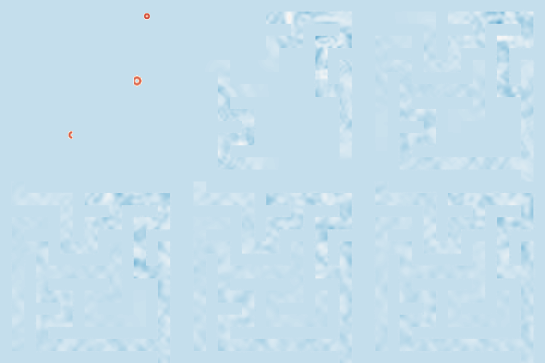
Example material densities can be seen below:

Traversal can be seen:

Dataset	FNO	TFNO	Unet	CNextU-net
acoustic_scattering_maze	0.5062	0.5057	0.0351	\(\mathbf{0.0153}\)

Table: VRMSE metrics on test sets (lower is better). Best results are shown in bold. VRMSE is scaled such that predicting the mean value of the target field results in a score of 1.

About the data

Dimension of discretized data: 201 steps of 256 \(\times\) 256 images.

Fields available in the data: pressure (scalar field), material density (constant scalar field), material speed of sound (constant scalar field), velocity field (vector field).

Number of trajectories: 2000.

Estimated size of the ensemble of all simulations: 311.3 GB.

Grid type: uniform, cartesian coordinates.

Initial conditions: Flat pressure static field with 1-6 high pressure rings randomly placed along paths of maze. The rings are defined with variable intensity \(\sim \mathcal U(3., 5.)\) and radius \(\sim \mathcal U(.01, .04)\). Any overlap with walls is removed.

Boundary conditions: Open domain in \(y\), reflective walls in \(x\).

Simulation time-step: Variable based on CFL with safety factor .25.

Data are stored separated by (\(\Delta t\)): 2/201.

Total time range (\(t_{min}\) to \(t_{max}\)): [0, 4.].

Spatial domain size (\(L_x\), \(L_y\)): [-1, 1] x [-1, 1].

Set of coefficients or non-dimensional parameters evaluated:

• \(K\) is fixed at 4.0.

• \(\rho\) is the primary coefficient here. We generated a maze with initial width between 6 and 16 pixels and upsample it via nearest neighbor resampling to create a 256 x 256 maze. The walls are set to \(\rho=10^6\) while paths are set to \(\rho=3\).

Approximate time to generate the data: ~20 minutes per simulation.

Hardware used to generate the data and precision used for generating the data: 64 Intel Icelake cores per simulation. Generated in double precision.

What is interesting and challenging about the data:

This is an example of simple dynamics in complicated geometry. The sharp discontinuities can be a significant problem for machine learning models, yet they are a common feature in many real-world physics. While visually the walls appear to stop the signal, it is actually simply the case that the speed of sound is much much lower inside the walls leading to partial reflection/absorbtion at the interfaces.

Please cite the associated paper if you use this data in your research:

@article{mandli2016clawpack,
  title={Clawpack: building an open source ecosystem for solving hyperbolic PDEs},
  author={Mandli, Kyle T and Ahmadia, Aron J and Berger, Marsha and Calhoun, Donna and George, David L and Hadjimichael, Yiannis and Ketcheson, David I and Lemoine, Grady I and LeVeque, Randall J},
  journal={PeerJ Computer Science},
  volume={2},
  pages={e68},
  year={2016},
  publisher={PeerJ Inc.}
}