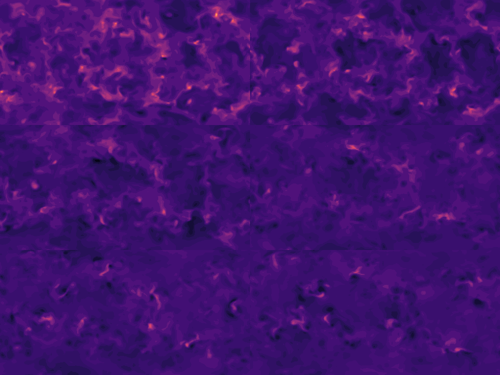
Red Supergiant Convective Envelope¶

One line description of the data: 3D radiation hydrodynamic simulations of the convective envelope of red supergiant stars.

Longer description of the data: Massive stars evolve into red supergiants, which have large radii and luminosities, and low-density, turbulent, convective envelopes. These simulations model the (inherently 3D) convective properties and gives insight into the progenitors of supernovae explosions.

Associated paper: Paper.

Domain experts: Yan-Fei Jiang (CCA, Flatiron Institute), Jared Goldberg (CCA, Flatiron Institute), Jeff Shen (Princeton University).

Code or software used to generate the data: Athena++.

Equations

\begin{align*}
\frac{\partial\rho}{\partial t}+\mathbf{\nabla}\cdot(\rho\mathbf{v})&=0\\
\frac{\partial(\rho\mathbf{v})}{\partial t}+\mathbf{\nabla}\cdot({\rho\mathbf{v}\mathbf{v}+{{\sf P_{\rm gas}}}}) &=-\mathbf{G}_r-\rho\mathbf{\nabla}\Phi \\
\frac{\partial{E}}{\partial t}+\mathbf{\nabla}\cdot\left[(E+ P_{\rm gas})\mathbf{v}\right] &= -c G^0_r -\rho\mathbf{v}\cdot\mathbf{\nabla}\Phi\\
\frac{\partial I}{\partial t}+c\mathbf{n}\cdot\mathbf{\nabla} I &= S(I,\mathbf{n})
\end{align*}

where

$\rho$ = gas density.
$\mathbf{v}$ = flow velocity.
${\sf P_{\rm gas}}$ = gas pressure tensor.
$P_{\rm gas}$ = gas pressure scalar.
$E$ = total gas energy density: $E = E_g + \rho v^2 / 2$, where $E_g = 3 P_{\rm gas} / 2$ = gas internal energy density.
$G^0_r$ and $\mathbf{G}_r$ = time-like and space-like components of the radiation four-force.
$I$ = frequency integrated intensity, which is a function of time, spatial coordinate, and photon propagation direction $\mathbf{n}$.
$\mathbf{n}$ = photon propagation direction.

Gif

Dataset	FNO	TFNO	Unet	CNextU-net
`convective_envelope_rsg`	$\mathbf{0.0269}$	0.0283	0.0555	0.0799

Table: VRMSE metrics on test sets (lower is better). Best results are shown in bold. VRMSE is scaled such that predicting the mean value of the target field results in a score of 1.

About the data¶

Dimension of discretized data: 100 time-steps of 256 $\times$ 128 $\times$ 256 images per trajectory.

Fields available in the data: energy (scalar field), density (scalar field), pressure (scalar field), velocity (vector field).

Number of trajectories: 29 (they are cuts of one long trajectory, long trajectory available on demand).

Estimated size of the ensemble of all simulations: 570 GB.

Grid type: spherical coordinates, uniform in $(\log r, \theta,\phi)$. Simulations are done for a portion of a sphere (not the whole sphere), so the simulation volume is like a spherical cake slice.

Initial and boundary conditions: The temperature at the inner boundary (IB) is first set to equal that of the appropriate radius coordinate in the MESA (1D) model ($400\~R_\odot$ and $300\~R_\odot$) and the density selected to approximately recover the initial total mass of the star in the simulation ($15.4\~M_\odot$ and $14\~M_\odot$). Between $300\~R_\odot$ and $400\~R_\odot$, the initial profile is constructed with the radiative luminosity to be $10^5\~L_\odot$, and this is kept fixed in the IB.

Simulation time-step: ~2 days.

Data are stored separated by ($\Delta t$): units here are sort of arbitrary, $\Delta t= 8$.

Total time range ($t_{min}$ to $t_{max}$): $t_{min} = 2$, $t_{max} = 23402$ (arbitrary).

Spatial domain size: $R$ from $300-6700~{\rm R_\odot}$, θ from $π/4−3π/4$ and $\phi$ from $0−π$, with $δr/r ≈ 0.01$.

Set of coefficients or non-dimensional parameters evaluated:

Simulation	radius of inner boundary $R_{IB}/R_\odot$	radius of outer boundary $R_{OB}/R_\odot$	heat source	resolution (r × θ × $\phi$)	duration	core mass $mc/M_\odot$	final mass $M_{\rm final}/M_\odot$
Whole simulation (to obtain the 29 trajectories)	300	6700	fixed L	256 × 128 × 256	5766 days	10.79	12.9

Approximate time to generate the data: 2 months on 80 nodes, or approximately 10 million CPU hours.

Hardware used to generate the data: 80x NASA Pleiades Skylake CPU nodes.

Additional information about the simulation: The radial extent of the simulation domain extends from $300~{\rm R_\odot}$ at the simulation inner boundary to $6700~{\rm R_\odot}$ at the simulation outer boundary, with logarithmic cell spacing in radius. The typical radius of the photosphere (or "surface") of the star is between $\approx 800 - 1000 ~{\rm R_\odot}$, fluctuating in space and time. Convection develops only at locations inside the star, within the first hundred radial zones or so. Some material from the star occasionally reaches larger radial distances. Outside of the stellar photosphere ("surface"), a density floor is set at $ \approx 10^{-16} g/cm^3$, and the material far outside the stellar photosphere generally reflects the infalling motion of gas and density floor material with very little mass, perturbed by the activity of the stellar surface. Additionally, because the temperature and density is very low, the opacities are not well-characterized in this material. So, while the RHD equations are still solved in this region of the simulation domain, one should not interpret things outside $\approx 1500 R_\odot$ as physically meaningful.

What is interesting and challenging about the data:¶

What phenomena of physical interest are captured in the data: turbulence and convection (inherently 3D processes), variability. Note that the stellar surface only extends out to roughly 1000 $R_\odot$, inside of which the interesting physics occurs.

How to evaluate a new simulator operating in this space: can it predict behaviour of simulation in convective steady-state, given only a few snapshots at the beginning of the simulation? can it properly model convection and turbulence?

Caveats: complicated geometry, size of a slice in R varies with R (think of this as a slice of cake, where the parts of the slice closer to the outside have more area/volume than the inner parts), simulation reaches convective steady-state at some point and no longer "evolves".

Please cite the associated paper if you use this data in your research:

@article{goldberg2022numerical,
  title={Numerical simulations of convective three-dimensional red supergiant envelopes},
  author={Goldberg, Jared A and Jiang, Yan-Fei and Bildsten, Lars},
  journal={The Astrophysical Journal},
  volume={929},
  number={2},
  pages={156},
  year={2022},
  publisher={IOP Publishing}
}