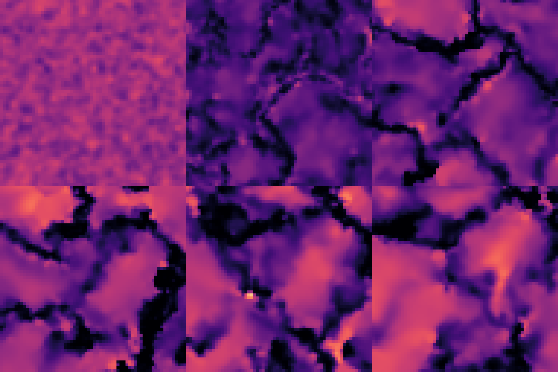
Turbulent Interstellar Medium in Galaxies¶

One line description of the data: Turbulence in an interstellar medium in various evolution stages of galaxies.

Longer description of the data: These simulations are a turbulent fluid with gravity modeling interstellar medium in galaxies. These fluids make dense filaments, which will form new stars. The timescale and frequency of making new filaments are varied depending on the strength of cooling. It is parametrized by the amount of metal (metallicity), density, and temperature.

Associated paper: Paper.

Domain expert: Keiya Hirashima, University of Tokyo & CCA, Flatiron Institute.

Code or software used to generate the data: ASURA-FDPS (Smoothed Particle Hydrodynamics), Github repository.

Equation:

\[ \begin{align*} P&=(\gamma-1) \rho u \\ \frac{d \rho}{dt} &= -\rho \nabla \cdot \mathbf{v} \\ \frac{d^2 \mathbf{r}}{dt^2} &= -\frac{\nabla P}{\rho} + \mathbf{a}_{\rm visc}-\nabla \Phi \\ \frac{d u}{dt} &= -\frac{P}{\rho} \nabla \cdot \mathbf{v} + \frac{\Gamma-\Lambda}{\rho} \end{align*} \]

where \(P\), \(\rho\), and \(u\) are the pressure. \(r\) is the position, \(a_{\rm visc}\) is the acceleration generated by the viscosity, \(\Phi\) is the gravitational potential, \(\Gamma\) is the radiative heat influx per unit volume, and \(\Lambda\) is the radiative heat outflux per unit volume.

Gif

Dataset	FNO	TFNO	Unet	CNextU-net
`turbulence_gravity_cooling`	0.2429	0.2673	0.6753	\(\mathbf{0.2096}\)

Table: VRMSE metrics on test sets (lower is better). Best results are shown in bold. VRMSE is scaled such that predicting the mean value of the target field results in a score of 1.

About the data¶

Dimension of discretized data: 50 time-steps of 64 \(\times\) 64 \(\times\) 64 cubes.

Fields available in the data: Pressure (scalar field), density (scalar field), temperature (scalar field), velocity (tensor field).

Number of trajectories: 2700 (27 parameters sets \(\times\) 100 runs).

Estimated size of the ensemble of all simulations: 829.4 GB.

Grid type: uniform, cartesian coordinates.

Initial conditions: 2700 random seeds generated using https://github.com/amusecode/amuse/blob/main/src/amuse/ext/molecular_cloud.py (Virialized isothermal gas sphere with turbulence following the velocity spectrum \(E(k) \propto k^{-2}\), which is Burgers turbulence (Burgers 1948 and Kupilas+2021 for reference)).

Boundary conditions: open.

Simulation time-step: \(2,000\) ~ \(10,000\) years (variable timesteps).

Data are stored separated by (\(\Delta t\)): 0.02 free fall time.

Total time range (\(t_{min}\) to \(t_{max}\)): 1 Free Fall time (= \(L^3/GM\) ); \(L=(\rho / \rho_0)^{1/3} \times 60\) pc, \(\rho_0=44.5/\rm{cc}\), \(M=1,000,000\) M \(_\odot\).

Spatial domain size (\(L_x\), \(L_y\), \(L_z\)):

	Domain Length (\(L\))	Free Fall Time	Snapshot (\(\delta t\))
Dense (44.5 cm \(^{-3}\))	60 pc	6.93 Myr	0.14 Myr
Moderate (4.45 cm \(^{-3}\))	129 pc	21.9 Myr	0.44 Myr
Sparse (0.445 cm \(^{-3}\))	278 pc	69.3 Myr	1.4 Myr

Set of coefficients or non-dimensional parameters evaluated: Initial temperature \(T_0=\{10K, 100K, 1000K\}\), Initial number density of hydrogen \(\rho_0=\{44.5/cc, 4.45/cc, 0.445/cc\}\), metallicity (effectively strength of cooling) \(Z=\{Z_0, 0.1\,Z_0, 0\}\).

Approximate time to generate the data: \(600\,000\) node hours for all simulations.

For dense dataset (CPU hours)¶

	Strong (1Z \(_\odot\))	Weak (0.1 Z \(_\odot\))	Adiabatic (0 Z \(_\odot\))
\(10\) K	\(240\)	\(167\)	\(77\)
\(100\) K	\(453\)	\(204\)	\(84\)
\(1000\) K	\(933\)	\(186\)	\(46\)

For moderate dataset (CPU hours)¶

	Strong (1Z \(_\odot\))	Weak (0.1 Z \(_\odot\))	Adiabatic (0 Z \(_\odot\))
\(10\) K	\(214\)	\(75\)	\(62\)
\(100\) K	\(556\)	\(138\)	\(116\)
\(1000\) K	\(442\)	\(208\)	\(82\)

For sparse dataset (CPU hours)¶

	Strong (1Z \(_\odot\))	Weak (0.1 Z \(_\odot\))	Adiabatic (0 Z \(_\odot\))
\(10\) K	\(187\)	\(102\)	\(110\)
\(100\) K	\(620\)	\(101\)	\(92\)
\(1000\) K	\(286\)	\(129\)	\(93\)

Hardware used to generate the data and precision used for generating the data: up to 1040 CPU cores per run.

What is interesting and challenging about the data:¶

What phenomena of physical interest are catpured in the data: Gravity, hydrodynamics and radiative cooling/heating are considered in the simulations. Radiative cooling/heating is parameterized with metallicity, which the ratio of heavier elements than helium. The larger and metallicity corresponds to the later and early stage of galaxies and universe, respectively. It also affects the time scale of cooling/heating and star formation rate. For instance, star formation happens at dense and cold region. With the strong cooling/heating rate, dense regions are quickly cooled down and generates new stars. Inversely, in the case of a weak cooling/heating, when gas is compressed, it is heated up and prevent new stars from being generated.

In the case of cold gas with strong cooling/heating, it can easily make dense regions, which require small timesteps and a lot of integration steps. That makes it difficult to get the resolution higher.

How to evaluate a new simulator operating in this space: The new simulator should be able to detect potential regions of star formation / potential number of newborn stars, because star formation regions are very dense and need very small timesteps, which results in a massive number of calculation steps.

Please cite the associated paper if you use this data in your research:

@article{hirashima20233d,
  title={3D-Spatiotemporal forecasting the expansion of supernova shells using deep learning towards high-resolution galaxy simulations},
  author={Hirashima, Keiya and Moriwaki, Kana and Fujii, Michiko S and Hirai, Yutaka and Saitoh, Takayuki R and Makino, Junichiro},
  journal={Monthly Notices of the Royal Astronomical Society},
  volume={526},
  number={3},
  pages={4054--4066},
  year={2023},
  publisher={Oxford University Press}
}